Backward SDEs-based Diffusion

TL;DR

A general framework that turns inverse problems into terminal-value problems: an associated BSDE composes any Score-SDE prior with a task-defined feasibility map, without retraining the score model.

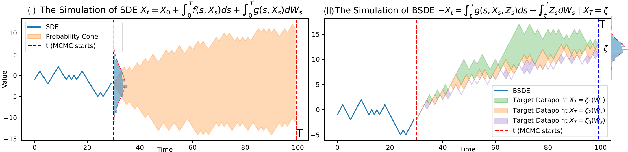
Reverse-time SDE sampling compared with an associated BSDE conditioned on a terminal target. — **Initial-value sampling versus terminal-value inversion.** Standard reverse-time SDEs begin from a reference noise law. Our associated BSDE begins with the endpoint requirement and solves for the adapted path.

Why a terminal condition?

In inverse problems, the output must be plausible and agree with a measurement $y=\mathcal{A}(x)+\eta$. Existing diffusion solvers often impose that agreement through guidance, repeated projection, or task-specific conditional training. These interventions act along the sampling path, but do not naturally express the requirement that matters most: feasibility at the end of inference.

Conventional diffusion solvers

Modify the path

Add measurement gradients, penalties, or projections at selected sampling steps.

Our perspective

Specify the endpoint

Encode feasibility as $Y_\tau=\Psi(y)$ and solve backward for an adapted prior state.

Key idea. Task information lives in the terminal map $\Psi$; the pretrained score-defined coefficients stay frozen.

An associated BSDE for a Score-SDE prior

Let a pretrained score model define the base stochastic dynamics $dX_t=b_\theta(X_t,t)dt+\sigma(t)dW_t$. For an observation $y$ and task-specific terminal map $\Psi$, we solve

$$Y_t=\Psi(y)+\int_t^\tau f_\theta(s,X_s,Y_s,Z_s)\,ds-\int_t^\tau Z_s\,dW_s.$$

Under standard Lipschitz and square-integrability conditions, the adapted solution $(Y,Z)$ exists and is unique. The recovered state $Y_0$ therefore gives a principled inverse map from the terminal requirement to the prior at the chosen noise level, while $Y_\tau=\Psi(y)$ enforces terminal consistency by construction.

Backward inversion recovers an anchored prior state and forward sampling produces feasible outputs. — **Backward inversion, forward generation.** The BSDE recovers an anchored prior state from the terminal specification. Score-based dynamics then turn that state into feasible reconstructions or nearby samples.

1

Connect any Score-SDE

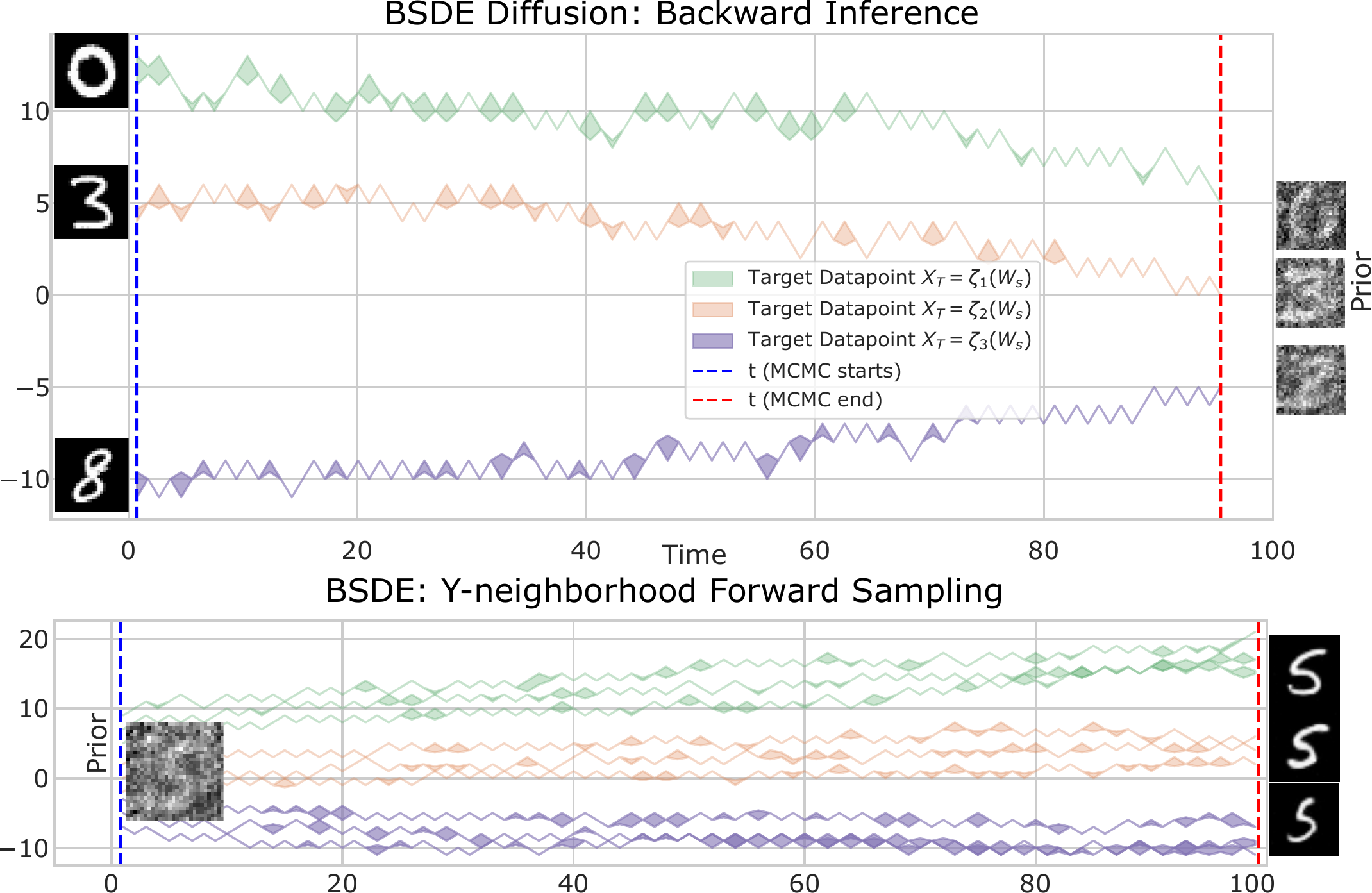
Expose the pretrained prior drift and diffusion without task-specific retraining.

2

Define task feasibility

Construct Ψ from the observation and the application's forward operator.

3

Solve and sample

Recover Y₀, generate feasible solutions, and probe its local uncertainty.

One case study · sparse-view CT

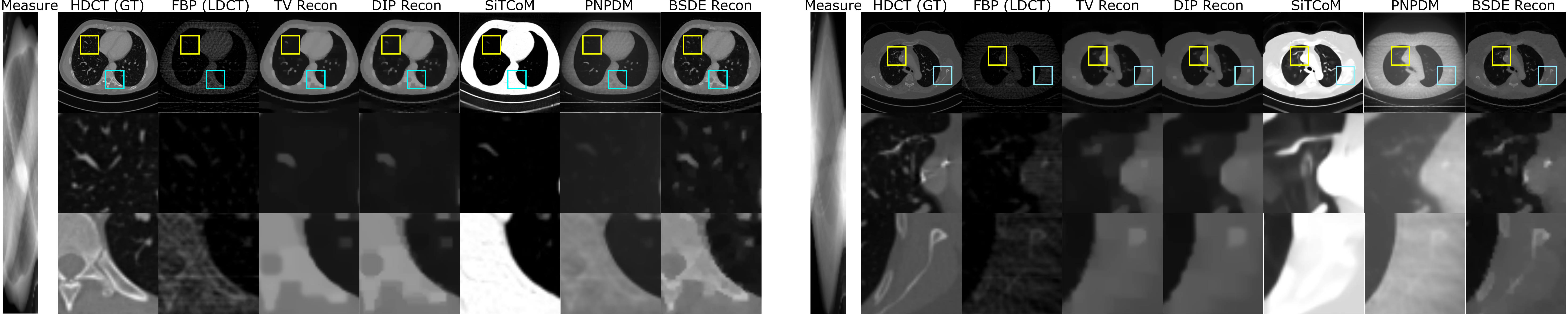
The framework instantiated with a CT terminal map

CT is an evaluation domain, not a framework dependency. Here, $\Psi$ decodes the prior state, enforces projection consistency, and re-encodes it. Other inverse problems replace only this task-owned map.

Low-dose CT examples comparing FBP, TV, DIP, SiTCoM, PnPDM, and the proposed BSDE reconstruction. — Two LDCT-to-HDCT examples. The BSDE reconstruction suppresses streak artifacts while preserving subtle lung textures and low-contrast structures; insets highlight fine pulmonary and bone detail.

3.57MAE ↓

30.99PSNR ↑

0.868SSIM ↑

0.0101NMSE ↓

0.989NCC ↑

Method	MAE ↓	PSNR ↑	SSIM ↑	NMSE ↓	NCC ↑
FBP	37.22	14.12	0.366	0.4695	0.902
TV	4.81	27.89	0.807	0.0205	0.978
DIP	4.56	28.08	0.816	0.0197	0.979
PnPDM	23.38	19.06	0.551	0.3531	0.934
SiTCoM	138.69	4.80	0.299	4.5928	0.975
BSDE (ours)	3.57	30.99	0.868	0.0101	0.989

Result. The proposed BSDE obtains the best reported value across all five reconstruction metrics in the manuscript table.

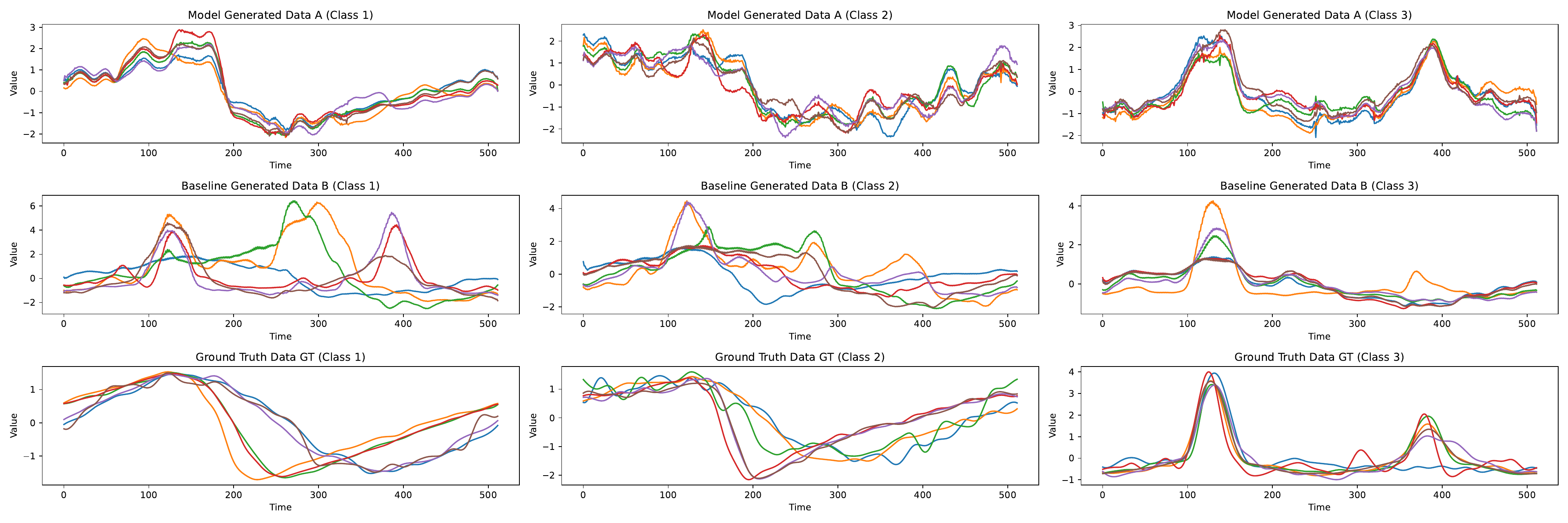
One inversion, a neighborhood of solutions

The recovered $Y_0$ is an anchor rather than a single deterministic answer. Perturbing it as $\widetilde{Y}_0=Y_0+\lambda\epsilon$ produces controlled diversity while preserving the shared terminal specification, making uncertainty accessible through local sampling in prior space.

MNIST terminal-controlled samples, target, recovered prior state, uncertainty mean, and uncertainty variance. — Repeated MNIST solves recover stable encodings. Nearby prior states preserve digit identity while Monte Carlo samples reveal spatial uncertainty.

Conditional generation of star lightcurves

Generated Cepheid, Eclipsing Binary, and RR Lyrae lightcurves for BSDE diffusion and baselines. — Neighborhood sampling across Cepheid, Eclipsing Binary, and RR Lyrae classes, compared with SDE diffusion, GAN inversion, LSTM-VAE, and target samples.

BibTeX

@inproceedings{wang2026backward,
  title     = {Backward SDEs-based Diffusion for Physics-Constrained Generation},
  author    = {Wang, Zihao},
  booktitle = {Proceedings of the 43rd International Conference on Machine Learning},
  series    = {Proceedings of Machine Learning Research},
  volume    = {306},
  publisher = {PMLR},
  year      = {2026}
}